Formatting cells in Google Sheets with Python

Introduction

One of the critical things that developers have not been able to do in previous versions of the Google Sheets API is to format cells... that's a big deal! Anyway, the past is the past, and I choose to look ahead. In my earlier post on the Google Sheets API, I introduced Sheets API v4 with a tutorial on how to transfer data from a SQL database to a Sheet. You'd do that primarily to make database data more presentable rather than deliberately switching to a storage mechanism with weaker querying capabilities. At the very end of that post, I challenged readers to try formatting. If you got stuck, confused, or haven't had a chance yet, today's your lucky day. One caveat is that there's more JavaScript in this post than Python... you've been warned!

Using the Google Sheets API

We need to write (formatting) into a Google Sheet, so we need the same scope as last time, read-write:

• 'https://www.googleapis.com/auth/spreadsheets' — Read-write access to Sheets and Sheet properties

Since we've fully covered the authorization boilerplate fully in earlier posts and videos, including how to connect to the Sheets API, we're going to skip that here and jump right to the action.

Formatting cells in Google Sheets

The way the API works, in general, is to take one or more commands, and execute them on the Sheet. This comes in the form of individual requests, either to cells, a Sheet, or the entire spreadsheet. A group if requests is organized as a JavaScript array. Each request in the array is represented by a JSON object. Yes, this part of the post may seem like a long exercise in JavaScript, but stay with me here. Continuing... once your array is complete, you send all the requests to the Sheet using the SHEETS.spreadsheets().batchUpdate() command. Here's pseudocode sending 5 commands to the API:

SHEET_ID =  . . .

reqs = {'requests': [
    {'updateSheetProperties':
        . . .
    {'repeatCell':
        . . .
    {'setDataValidation':
        . . .
    {'sortRange':
        . . .
    {'addChart':
        . . .
]}
SHEETS.spreadsheets().batchUpdate(
        spreadsheetId=SHEET_ID, body=reqs).execute()

What we're executing will be similar. The target spreadsheet will be the one you get when you run the code from the previous post, only without the timestamp in its title as it's unnecessary:


Once you've run the earlier script and created a Sheet of your own, be sure to assign it to the SHEET_ID variable. The goal is to send enough formatting commands to arrive at the same spreadsheet but with improved visuals: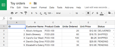


Four (4) requests are needed to bring the original Sheet to this state:

1. Set the top row as "frozen", meaning it doesn't scroll even when the data does
2. Also bold the first row, as these are the column headers
3. Format column E as US currency with dollar sign & 2 decimal places
4. Set data validation for column F, requiring values from a fixed set

Creating Sheets API requests

As mentioned before, each request is represented by a JSON object, cleverly disguised as Python dictionaries in this post, and the entire request array is implemented as a Python list. Let's take a look at what it takes to together the individual requests:

Frozen rows

Frozen rows is a Sheet property, so in order to change it, users must employ the updateSheetProperties command. Specifically, frozenRowCount is a grid property, meaning the field that must be updated is gridProperties.frozenRowCount, set to 1. Here's the Python dict (that gets converted to a JSON object) representing this request:

{'updateSheetProperties': {
    'properties': {'gridProperties': {'frozenRowCount': 1}},
    'fields': 'gridProperties.frozenRowCount',
}},

The properties attribute specifies what is changing and what the new value is. The fields property serves as an attribute "mask." It's how you specify what to alter and what to leave alone when applying a change. In this case, both the properties and fields attributes refer to the same thing: the frozen row count grid property. If you leave out the fields attribute here, sure the frozen row count would be set but all other grid properties would be undone, not such a good side effect. It's okay if it doesn't make a lot of sense yet... there are more examples coming.

Bold formatting

Text formatting, such as bold or italics, is a cell operation. Since we want to apply this formatting to multiple cells, the correct command is, repeatCell. Specifically, what needs to be changed about a cell? A cell's userEnteredFormat.textFormat.bold attribute. This is a simple Boolean value, so we set it to True. The fields masks are as described above... we need to tell the API to explicitly change the just userEnteredFormat.textFormat.bold attribute. Everything else should stay as-is.

The last thing we need is to tell the API which cells in the Sheet should be formatted. For this we have range. This attribute tells the API what Sheet (by ID) and which cells (column and row ranges) in that Sheet to format. Above, you see that we want to bold just one row, row #1. Similarly, there are currently six columns to bold, A-F.

However, like most modern computer systems, the API supports start and end index values beginning with zero... not alphabetic column names nor rows consisting of whole numbers, and the range is exclusive of the end index, meaning it goes up to but does not include the ending row or column. For row 1, this means a starting index of 0 and an ending index of 1. Similarly, columns A-F have start & end index value of 0 and 6, respectively. Visually, here's how you compare traditional row & column values to 0-based index counting:


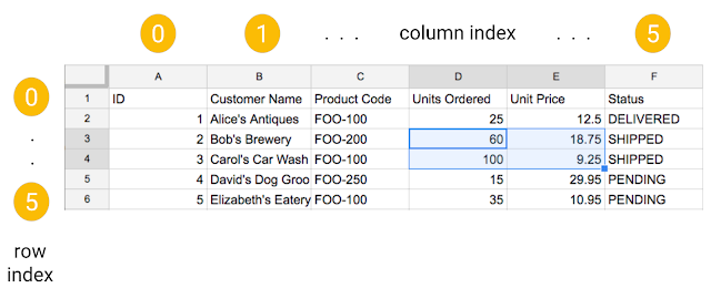
Here's the dict representing this request:

{'repeatCell': {
    'range': {
        'sheetId': 0,
        'startColumnIndex': 0,
        'endColumnIndex': 6,
        'startRowIndex': 0,
        'endRowIndex': 1
    },
    'cell': {'userEnteredFormat': {'textFormat': {'bold': True}}},
    'fields': 'userEnteredFormat.textFormat.bold',
}},

Before we move on, let's talk about some shortcuts we can make. The ID of the first Sheet created for you is 0. If that's the Sheet you're using, then you can omit passing the Sheet ID. Similarly, the starting row and column indexes default to 0, so you can leave those out too if those are the values to be used. Finally, while an ending column index of 6 works, it won't if more columns are added later. It's best if you just omit the ending index altogether, meaning you want that entire row formatted. All this means that the only thing in the range you need is the ending row index. Instead of the above, your request can be shortened to:

{'repeatCell': {
    'range': {'endRowIndex': 1},
    'cell': {'userEnteredFormat': {'textFormat': {'bold': True}}},
    'fields': 'userEnteredFormat.textFormat.bold',
}},

Range quiz

Okay, now that you know about ranges, take this quiz: assumming the Sheet ID is 0, what are the starting and ending column and row indexes for the four cells highlighted in blue in this Sheet?


If you went with starting and ending column indexes of 3 and 5 and row indexes of 2 and 4, then you're right on the money and ready for more!

Currency formatting

Currency formatting is similar to text formatting, only with numbers, meaning that instead of userEnteredFormat.textFormat, you'd be setting a cell's userEnteredFormat.numberFormat attribute. The command is also repeatCell. Clearly the starting and ending column indexes should be 4 and 5 with a starting row index of 1. But just like the cell bolding we did above, there's no need to restrict ourselves to just the 5 rows of data as more may be coming. Yes, it's best to leave off the ending row index so that the rest of the column is formatted. The only thing you need to learn is how to format cells using US currency, but that's pretty easy to do after a quick look at the docs on formatting numbers:

{'repeatCell': {
    'range': {
        'startRowIndex': 1,
        'startColumnIndex': 4,
        'endColumnIndex': 5,
    },
    'cell': {
        'userEnteredFormat': {
            'numberFormat': {
                'type': 'CURRENCY',
                'pattern': '"$"#,##0.00',
            },
        },
    },
    'fields': 'userEnteredFormat.numberFormat',
}}

More on fields

One caveat to our sample app here is that all of the fields mask only have a single value, the one we want to change, but that's not always the case. There may be situations where you want to effect a variety of changes to cells. To see more examples of fields, check out this page in the docs featuring more formatting examples. To learn more about how masking works, check out this page and this one too.

Cell validation

The final formatting request implements cell validation on column F as well as restricting their possible values. The command used here is setDataValidation. The range is similar to that of currency formatting, only for column F, meaning a starting row index of 1, and starting and ending column indexes of 5 and 6, respectively. The rule implements the restriction. Similar to other spreadsheet software, you can restrict cell values in any number of ways, as outlined by the ConditionType documentation page. Ours is to allow for one of three possible values, so the ConditionType is ONE_OF_LIST.

When you restrict cell values, you can choose to allow but flag it (weak enforcement) or disallow any value outside of what you specify (strict enforcement). If you wish to employ strict enforcement, you need to pass in a strict attribute with a True value. The default is weak enforcement, or False. In either case, users entering invalid values will get a default warning message that the input is not allowed. If you prefer a custom message over the default option, you can pass that to the API as the inputMessage attribute. I prefer the system default and elect not to use it here. Here are the 4 combinations of what shows up when you use or don't use inputMessage with strict and weak enforcement: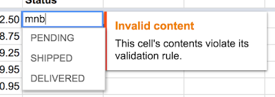


No inputMessage (default) + weak enforcement


With inputMessage (my custom msg) + weak enforcement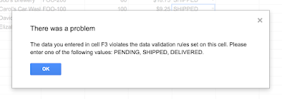


No inputMessage (default) + strict enforcement


With inputMessage (my custom msg) + weak enforcement

The last attribute you can send is showCustomUi. If the showCustomUi flag is set to True, the Sheets user interface will display a small pulldown menu listing the values accepted by the cell. It's a pretty poor user experience without it (because users won’t know what the available choices are), so I recommend you always use it too. With that, this request looks like this:

{'setDataValidation': {
    'range': {
        'startRowIndex': 1,
        'startColumnIndex': 5,
        'endColumnIndex': 6,
    },
    'rule': {
        'condition': {
            'type': 'ONE_OF_LIST',
            'values': [
                {'userEnteredValue': 'PENDING'},
                {'userEnteredValue': 'SHIPPED'},
                {'userEnteredValue': 'DELIVERED'},
            ]
        },
        #'inputMessage': 'Select PENDING, SHIPPED, or DELIVERED',
        #'strict': True,
        'showCustomUi': True,
    },
}}

Since we're not modifying cell attributes, but instead focusing on validation, you'll notice there's no fields mask in these types of requests.

Running our script

Believe it or not, that's the bulk of this application. With the reqs list of these four requests, the last line of code calls the Sheets API exactly like the pseudocode above. Now you can simply run it:

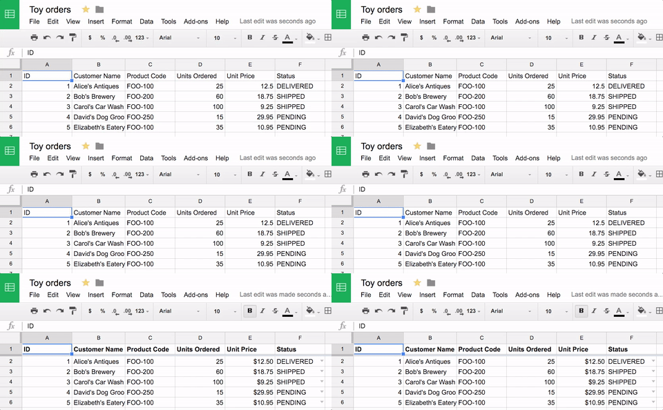
$ python sheets_cell_format.py # or python3
$

There's no output from this script, so you should only expect that your Sheet will be formatted once it has completed. If you bring up the Sheet in the user interface, you should see the changes happening in near real-time:

Conclusion

Below is the entire script for your convenience which runs on both Python 2 and Python 3 (unmodified!):

from apiclient import discovery
from httplib2 import Http
from oauth2client import file, client, tools

SCOPES = 'https://www.googleapis.com/auth/spreadsheets'
store = file.Storage('storage.json')
creds = store.get()
if not creds or creds.invalid:
    flow = client.flow_from_clientsecrets('client_id.json', SCOPES)
    creds = tools.run_flow(flow, store)
SHEETS = discovery.build('sheets', 'v4', http=creds.authorize(Http()))

SHEET_ID = ... # add your Sheet ID here
reqs = {'requests': [
    # frozen row 1
    {'updateSheetProperties': {
        'properties': {'gridProperties': {'frozenRowCount': 1}},
        'fields': 'gridProperties.frozenRowCount',
    }},
    # embolden row 1
    {'repeatCell': {
        'range': {'endRowIndex': 1},
        'cell': {'userEnteredFormat': {'textFormat': {'bold': True}}},
        'fields': 'userEnteredFormat.textFormat.bold',
    }},
    # currency format for column E (E2:E7)
    {'repeatCell': {
        'range': {
            'startRowIndex': 1,
            'endRowIndex': 6,
            'startColumnIndex': 4,
            'endColumnIndex': 5,
        },
        'cell': {
            'userEnteredFormat': {
                'numberFormat': {
                    'type': 'CURRENCY',
                    'pattern': '"$"#,##0.00',
                },
            },
        },
        'fields': 'userEnteredFormat.numberFormat',
    }},
    # validation for column F (F2:F7)
    {'setDataValidation': {
        'range': {
            'startRowIndex': 1,
            'endRowIndex': 6,
            'startColumnIndex': 5,
            'endColumnIndex': 6,
        },
        'rule': {
            'condition': {
                'type': 'ONE_OF_LIST',
                'values': [
                    {'userEnteredValue': 'PENDING'},
                    {'userEnteredValue': 'SHIPPED'},
                    {'userEnteredValue': 'DELIVERED'},
                ]
            },
            #'inputMessage': 'Select PENDING, SHIPPED, or DELIVERED',
            #'strict': True,
            'showCustomUi': True,
        },
    }},
]}

res = SHEETS.spreadsheets().batchUpdate(
        spreadsheetId=SHEET_ID, body=reqs).execute()

As with our other code samples, you can now customize for your own needs, for a mobile frontend, sysadmin script, or a server-side backend, perhaps accessing other Google APIs.

Code challenge

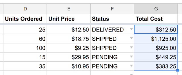
Once you fully grasp this sample and are ready for a challenge: Use the API to create a column "G" with a "Total Cost" header in cell G1, set cell G2 with the formula to calculate the cost based on toys ordered & cost in columns D & E then and create an autoFill request to replicate that formula down column G. When you're done, the right-hand side of your Sheet now looks like this:

Here are some steps you can take to achieve this improvement:

1. Create column G with a "Total Cost" header in cell G1; make sure it's bold too (or do you have to?)
2. Set cell G2 with formula =MULTIPLY(D2,E2)
3. Use autoFill command to copy formula from G2 down the entire column (HINT: you only need the range attribute)

You're now well under way to being able to writing useful applications with the Sheets API!